This repo demonstrates how to download and use OD data from Spain, published by transportes.gob.es
The data is provided as follows:
- Estudios basicos
- Por disitritos
- Personas (population)
- Pernoctaciones (overnight stays)
- Viajes
- ficheros-diarios
- meses-completos
- Por disitritos
The package is designed to save people time by providing the data in analyis-ready formats. Automating the process of downloading, cleaning and importing the data can also reduce the risk of errors in the laborious process of data preparation.
The datasets are large, so the package aims to reduce computational resources, by using computationally efficient packages behind the scenes. If you want to use many of the data files, it’s recommended you set a data directory where the package will look for the data, only downloading the files that are not already present.
Set the data directory by setting the SPANISH_OD_DATA_DIR environment variable, e.g. the following command:
usethis::edit_r_environ()
# Then set the data director, by typing this line in the file:
if (!requireNamespace("remotes", quietly = TRUE)) {
  install.packages("remotes")
}
remotes::install_cran("duckdb")
library(duckdb)
library(tidyverse)
theme_set(theme_minimal())
devtools::load_all()
sf::sf_use_s2(FALSE)
Get metadata for the datasets as follows:
metadata = get_metadata()
metadata
# A tibble: 8,453 × 6
target_url pub_ts file_extension data_ym data_ymd
<chr> <dttm> <chr> <date> <date>
1 https://movilidad-o… 2024-05-16 09:00:45 tar NA NA
2 https://movilidad-o… 2024-05-16 08:58:20 tar NA NA
3 https://movilidad-o… 2024-05-16 08:58:18 tar NA NA
4 https://movilidad-o… 2024-05-16 08:57:24 tar NA NA
5 https://movilidad-o… 2024-05-16 08:55:49 tar NA NA
6 https://movilidad-o… 2024-05-16 08:55:47 tar NA NA
7 https://movilidad-o… 2024-05-16 08:55:10 tar NA NA
8 https://movilidad-o… 2024-05-16 08:54:13 tar NA NA
9 https://movilidad-o… 2024-05-16 08:54:11 tar NA NA
10 https://movilidad-o… 2024-05-16 08:52:26 tar NA NA
# ℹ 8,443 more rows
# ℹ 1 more variable: local_path <chr>Zones
Zones can be downloaded as follows:
distritos = get_zones(type = "distritos")
distritos_wgs84 = sf::st_transform(distritos, 4326)
plot(distritos_wgs84)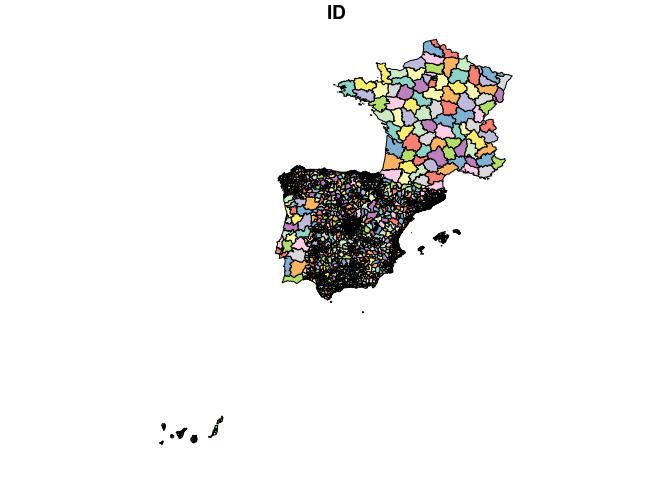
Estudios basicos
Each day in the ficheros-diarios folder contains a file with the following columns:
# set timeout for downloads
options(timeout = 600) # 10 minutes
u1 = "https://movilidad-opendata.mitma.es/estudios_basicos/por-distritos/viajes/ficheros-diarios/2024-03/20240301_Viajes_distritos.csv.gz"
f1 = basename(u1)
if (!file.exists(f1)) {
  download.file(u1, f1)
}
drv = duckdb::duckdb("daily.duckdb")
con = DBI::dbConnect(drv)
od1 = duckdb::tbl_file(con, f1)
# colnames(od1)
#  [1] "fecha"                   "periodo"
#  [3] "origen"                  "destino"
#  [5] "distancia"               "actividad_origen"
#  [7] "actividad_destino"       "estudio_origen_posible"
#  [9] "estudio_destino_posible" "residencia"
# [11] "renta"                   "edad"
# [13] "sexo"                    "viajes"
# [15] "viajes_km"
od1_head = od1 |>
  head() |>
  collect()
od1_head |>
knitr::kable()| fecha | periodo | origen | destino | distancia | actividad_origen | actividad_destino | estudio_origen_posible | estudio_destino_posible | residencia | renta | edad | sexo | viajes | viajes_km |
|---|---|---|---|---|---|---|---|---|---|---|---|---|---|---|
| 20240301 | 19 | 01009_AM | 01001 | 0.5-2 | frecuente | casa | no | no | 01 | 10-15 | NA | NA | 5.124 | 6.120 |
| 20240301 | 15 | 01002 | 01001 | 10-50 | frecuente | casa | no | no | 01 | 10-15 | NA | NA | 2.360 | 100.036 |
| 20240301 | 00 | 01009_AM | 01001 | 10-50 | frecuente | casa | no | no | 01 | 10-15 | NA | NA | 1.743 | 22.293 |
| 20240301 | 05 | 01009_AM | 01001 | 10-50 | frecuente | casa | no | no | 01 | 10-15 | NA | NA | 2.404 | 24.659 |
| 20240301 | 06 | 01009_AM | 01001 | 10-50 | frecuente | casa | no | no | 01 | 10-15 | NA | NA | 5.124 | 80.118 |
| 20240301 | 09 | 01009_AM | 01001 | 10-50 | frecuente | casa | no | no | 01 | 10-15 | NA | NA | 7.019 | 93.938 |
DBI::dbDisconnect(con)You can get the same result, but for multiple files, as follows:
od_multi_list = get_od(
  subdir = "estudios_basicos/por-distritos/viajes/ficheros-diarios",
  date_regex = "2024-03-0[1-7]"
)
od_multi_list[[1]]
# Source: SQL [?? x 15]
# Database: DuckDB v0.10.2 [robin@Linux 6.5.0-35-generic:R 4.4.0/:memory:]
fecha periodo origen destino distancia actividad_origen actividad_destino
<dbl> <chr> <chr> <chr> <chr> <chr> <chr>
1 20240307 00 01009_… 01001 0.5-2 frecuente casa
2 20240307 09 01009_… 01001 0.5-2 frecuente casa
3 20240307 18 01009_… 01001 0.5-2 frecuente casa
4 20240307 19 01009_… 01001 0.5-2 frecuente casa
5 20240307 20 01009_… 01001 0.5-2 frecuente casa
6 20240307 14 01002 01001 10-50 frecuente casa
7 20240307 22 01002 01001 10-50 frecuente casa
8 20240307 06 01009_… 01001 10-50 frecuente casa
9 20240307 09 01009_… 01001 10-50 frecuente casa
10 20240307 11 01009_… 01001 10-50 frecuente casa
# ℹ more rows
# ℹ 8 more variables: estudio_origen_posible <chr>,
# estudio_destino_posible <chr>, residencia <chr>, renta <chr>, edad <chr>,
# sexo <chr>, viajes <dbl>, viajes_km <dbl>
class(od_multi_list[[1]])The result is a list of duckdb tables which load almost instantly, and can be used with dplyr functions. Let’s do an aggregation to find the total number trips per hour over the 7 days:
n_per_hour = od_multi_list |>
  map(~ .x |>
        group_by(periodo, fecha) |>
        summarise(n = n(), Trips = sum(viajes)) |>
        collect()
  ) |>
  list_rbind() |>
  mutate(Time = lubridate::ymd_h(paste0(fecha, periodo))) |>
  mutate(Day = lubridate::wday(Time, label = TRUE))
n_per_hour |>
  ggplot(aes(x = Time, y = Trips)) +
  geom_line(aes(colour = Day)) +
  labs(title = "Number of trips per hour over 7 days")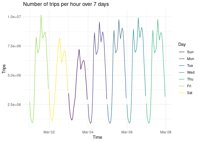
The figure above summarises 925,874,012 trips over the 7 days associated with 135,866,524 records.
We’ll use the same input data to pick-out the most important flows in Spain, with a focus on longer trips for visualisation:
od_large = od_multi_list |>
  map(~ .x |>
        group_by(origen, destino) |>
        summarise(Trips = sum(viajes), .groups = "drop") |>
        filter(Trips > 500) |>
        collect()
  ) |>
  list_rbind() |>
  group_by(origen, destino) |>
  summarise(Trips = sum(Trips)) |>
  arrange(desc(Trips))
od_large
# A tibble: 37,023 × 3
# Groups: origen [3,723]
origen destino Trips
<chr> <chr> <dbl>
1 2807908 2807908 2441404.
2 0801910 0801910 2112188.
3 0801902 0801902 2013618.
4 2807916 2807916 1821504.
5 2807911 2807911 1785981.
6 04902 04902 1690606.
7 2807913 2807913 1504484.
8 2807910 2807910 1299586.
9 0704004 0704004 1287122.
10 28106 28106 1286058.
# ℹ 37,013 more rowsThe results show that the largest flows are intra-zonal. Let’s keep only the inter-zonal flows:
od_large_interzonal = od_large |>
  filter(origen != destino)
We can convert these to geographic data with the {od} package:
od_large_interzonal_sf = od::od_to_sf(
  od_large_interzonal,
  z = distritos_wgs84
)
od_large_interzonal_sf |>
  ggplot() +
  geom_sf(aes(size = Trips), colour = "red") +
  theme_void()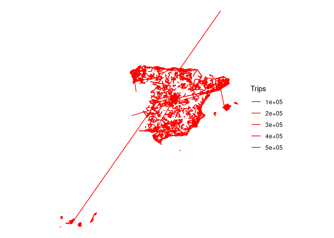
Let’s focus on trips in and around a particular area (Salamanca):
salamanca_zones = zonebuilder::zb_zone("Salamanca")
distritos_salamanca = distritos_wgs84[salamanca_zones, ]
plot(distritos_salamanca)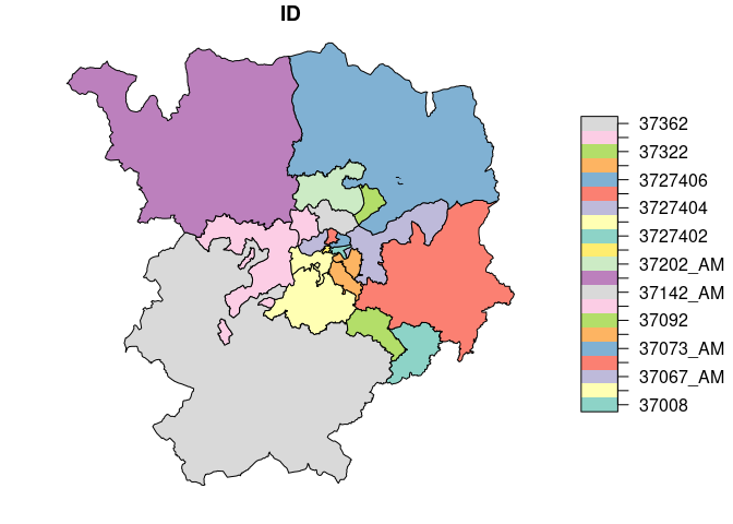
We will use this information to subset the rows, to capture all movement within the study area:
ids_salamanca = distritos_salamanca$ID
od_salamanca = od_multi_list |>
  map(~ .x |>
        filter(origen %in% ids_salamanca) |>
        filter(destino %in% ids_salamanca) |>
        collect()
  ) |>
  list_rbind() |>
  group_by(origen, destino) |>
  summarise(Trips = sum(viajes)) |>
  arrange(Trips)
Let’s plot the results:
od_salamanca_sf = od::od_to_sf(
  od_salamanca,
  z = distritos_salamanca
)
od_salamanca_sf |>
  filter(origen != destino) |>
  ggplot() +
  geom_sf(aes(colour = Trips), size = 1) +
  scale_colour_viridis_c() +
  theme_void()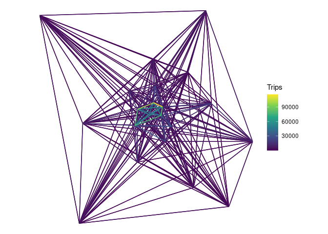
Disaggregating desire lines
For this you’ll need some additional dependencies:
We’ll get the road network from OSM:
salamanca_boundary = sf::st_union(distritos_salamanca)
osm_full = osmactive::get_travel_network(salamanca_boundary)
osm = osm_full[salamanca_boundary, ]
drive_net = osmactive::get_driving_network(osm)
drive_net_major = osmactive::get_driving_network_major(osm)
cycle_net = osmactive::get_cycling_network(osm)
cycle_net = osmactive::distance_to_road(cycle_net, drive_net_major)
cycle_net = osmactive::classify_cycle_infrastructure(cycle_net)
map_net = osmactive::plot_osm_tmap(cycle_net)
map_net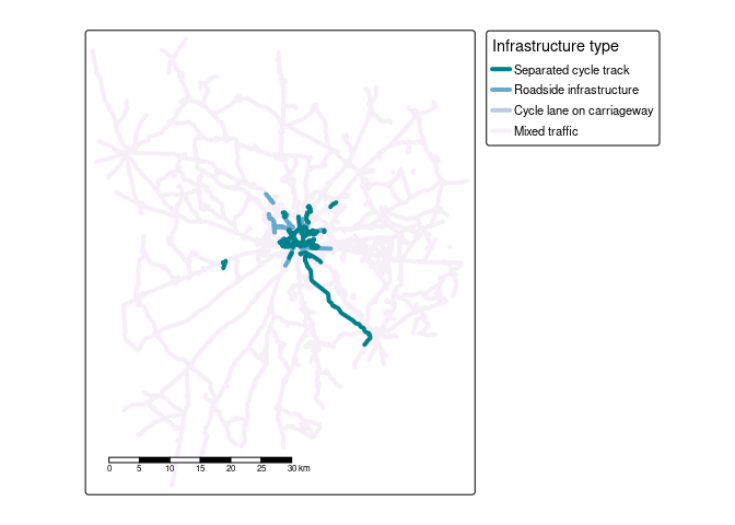
We can use the road network to disaggregate the desire lines:
od_jittered = odjitter::jitter(
od_salamanca_sf,
zones = distritos_salamanca,
subpoints = drive_net,
disaggregation_threshold = 1000,
disaggregation_key = "Trips"
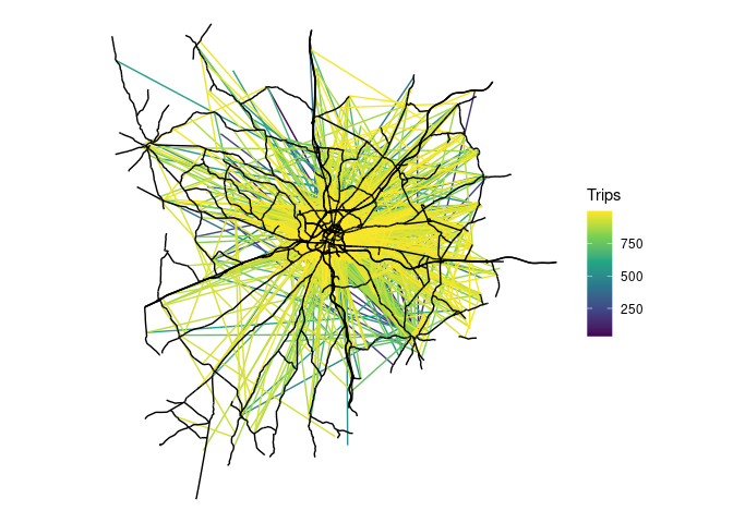
)Let’s plot the disaggregated desire lines:
od_jittered |>
  arrange(Trips) |>
  ggplot() +
  geom_sf(aes(colour = Trips), size = 1) +
  scale_colour_viridis_c() +
  geom_sf(data = drive_net_major, colour = "black") +
  theme_void()